About a year ago, Jim Bullard criticized the argument that that the Fed was missing on both sides of its dual mandate. Mark Sadowski (who should have his own blog, I think) has asked me to post his reply. I am most happy to do so.
=======================================
=======================================
This
is written in response to a question David Andolfatto posed in September in a
blog post entitled “Is the Fed missing on both sides of its dual mandate?”
David
concluded that post with the following statement:
“Bullard suggests that a non-monotonic
transition path for inflation is unlikely to be part of any optimal path in a
NK [New Keynesian] type model. The optimal path for inflation is unlikely to be
part of any optimal path in a NK type model. The optimal transition dynamics are
typically monotonic—think of the optimal transition path as a movement back up
the PC [Phillips Curve] in the diagram above. If this is true, then the optimal
transition path necessarily has the Fed missing on both sides of its dual
mandate.
Of course, conventional NK models frequently abstract from a
lot of considerations that many people feel are important for understanding the
recent recession and sluggish recovery. The optimal monetary policy may indeed
dictate "inflation overshooting" in a different class of models.
Please feel free to put forth your favorite candidate. Tell me why you think Bullard
is wrong.”
James
Bullard, President of the St. Louis Fed, had just written an opinion piece for
the Financial Times where he stated:
“To
argue against monotonic convergence now would imply that when unemployment is
above the natural rate, monetary policy should aim for inflation above the
Fed’s 2 per cent target. On the face of it, this does not make sense: the US
has experienced periods when both inflation and unemployment have been above
desirable levels. In the 1970s this phenomenon was labeled stagflation.
Monetary policy has been regarded as poor during that period.”
At
the time Scott Sumner mockingly responded:
“To
argue for monotonic convergence now would imply that when unemployment is above
the natural rate, monetary policy should aim for inflation below the Fed’s 2
per cent target. On the face of it, this does not make sense: the US has
experienced periods when both inflation and employment have been below
desirable levels. In the 1930s this phenomenon was labeled “The Great
Depression.” Monetary policy has been regarded as poor during that period.”
Sumner
is of course talking about the contractionary portion of the U.S. Great
Depression. The subsequent 1933-37 recovery, during which real GDP grew at an
average rate of 9.5%, is an excellent example of “oscillatory convergence” with
unemployment high and falling and inflation higher than normal. And yes, monetary
policy is generally regarded as excellent during that period.
Andolfatto’s,
Bullard’s, and Sumner’s comments raise a great many questions. For example, what
is the relationship between unemployment and inflation? How has this
relationship changed over time, and why? How has this relationship been modeled
over time? How should this relationship affect the conduct of monetary policy? For
the moment, at least, I want to stay focused on Bullard’s remarks.
As
evidence Bullard cited a paper by Frank Smets and Raf Wouters, “Shocks and
Frictions in US Business Cycles – A Bayesian DSGE Approach” (American Economic
Review, Vol. 97, No. 3, June 2007, pp. 566-606). In an essay published about a
month later, “Monetary Policy and the Expected Adjustment Path of Key
Variables” (Federal Reserve Bank of St. Louis Economic Synopses, 2012, No. 30),
Bullard clarified his Financial Times comments:
“Let’s
consider the medium-sized macroeconomic framework of Smets and Wouters (2007).
This is an important benchmark model; and, while we could argue about the
details, I think it will serve to make my point. In the Smets and Wouters
dynamic stochastic general equilibrium (DSGE) model there are many shocks, and
there is a monetary policymaker that follows a Taylor-type monetary policy rule
not unlike ones used in actual policy discussions. The authors estimate their
model using postwar U.S. data, and they also report results for subsamples
including the post-1984 data. Importantly, what the authors are estimating is a
general equilibrium for the economy, which includes monetary policy.
How
does the economy adjust in the Smets and Wouters model? The chart is Figure 2
from their paper.
The
authors plot the reaction of key macroeconomic variables to three types of
shocks in their model that might be thought of as demand shocks. Variables are
reported as deviations from a steady-state value, so that zero represents a
return to normal. The variables include inflation and a labor market
variable—hours worked. Time is measured in quarters. The shock is a positive
one—output and hours go up in response—but the story is merely transposed for a
negative shock (i.e., flip the figures upside down).
The
reaction of all variables is essentially monotonic beyond the hump in these
graphs, at least through year four. (That is, the adjustment does not show much
of a tendency to oscillate about the long-run value.) For all three types of
demand shocks, the Fed would be “missing on both sides of the dual mandate”
almost all of the time as the economy recovers from the shock. If the shock
were negative, hours would be too low (unemployment too high), and inflation
would be too low every quarter for many years. Yet the monetary policy embedded
in this general equilibrium is a Taylor-type policy rule that has often been
argued to closely approximate the optimal monetary policy in frameworks such as
this one. 2 It is in this sense that I do not think merely observing where
inflation and unemployment are relative to targets or long-run levels at a
point in time is telling us very much about whether the monetary policy in use
is the appropriate one or not.”
Footnote
2 reads:
“One
can investigate optimal-control monetary policy assuming credible commitment in
this model, taking the non-policy parameters as estimated by Smets and Wouters.
This type of monetary policy changes these impulse response functions but still
leaves goal variables “missing on both sides of the mandate” in many
situations. I thank Robert Tetlow for investigating this issue in response to
an earlier draft.”
The
monetary policy reaction function that is built into the Smets and Wouters
(2007) model is the original rule John Taylor proposed in 1993 ("Discretion
versus Policy Rules in Practice", Carnegie-Rochester Conference Series on Public
Policy, Vol. 39, December 1993, pp. 195-214), namely a Taylor Rule that places
equal weights on the inflation gap and the output gap. In 1999 Taylor discussed
an alternative version of this rule that placed double the weight on the output
gap than on the inflation gap, (“A Historical Analysis of Monetary Policy
Rules”, Monetary Policy Rules, Chicago: University of Chicago Press, pp.
319-341). This is a point to which we shall return later. Thus the response of
the economy to the demand shocks illustrated in Figure 2 is conditional on the
Taylor Rule embedded in the model.
At
this point it might be worth mentioning that one of the acknowledged
shortcomings of medium-scale New Keynesian DSGE models is that typically there
is no reference to unemployment. Bullard infers the impact of a demand shock on
unemployment from its effect on hours worked. In particular, the Phillips Curve
in the Smets-Wouters model is a hybrid New Keynesian type in which inflation
depends on past inflation, expected future inflation, current price mark-up and
a price mark-up disturbance. Apparently the only reference in the model to the
output gap occurs in the model’s monetary policy reaction function (i.e. the
Taylor Rule).
Bullard’s
footnote on optimal control monetary policy is especially relevant in this
context. What is “optimal control” monetary policy? Federal Reserve Vice Chair
Janet Yellen spoke about optimal control techniques in speeches in April, June
and November of last year. Here is how she introduced them in April:
“One
approach I find helpful in judging an appropriate path for policy is based on
optimal control techniques. Optimal control can be used, under certain
assumptions, to obtain a prescription for the path of monetary policy
conditional on a baseline forecast of economic conditions. Optimal control
typically involves the selection of a particular model to represent the
dynamics of the economy as well as the specification of a "loss
function" that represents the social costs of deviations of inflation from
the Committee's longer-run goal and of deviations of unemployment from its
longer-run normal rate. In effect, this approach assumes that the policymaker
has perfect foresight about the evolution of the economy and that the private
sector can fully anticipate the future path of monetary policy; that is, the central
bank's plans are completely transparent and credible to the public."
In
that speech Yellen describes how projections generated by FRB/US, the Federal
Reserve’s primary forecasting model, were adjusted to replicate the baseline outlook
constructed using the distribution of FOMC participants' projections for
unemployment, inflation, and the federal funds rate that were published in
January of that year. A search procedure was used to solve for the path of the
federal funds rate that minimized the value of a loss function. The loss
function was equal to the cumulative sum from 2012:Q2 through 2025:Q4 of three
factors: 1) the discounted squared deviation of the unemployment rate from
5-1/2 percent, 2) the squared deviation of overall PCE inflation from 2
percent, and 3) the squared quarterly change in the federal funds rate. She
termed this path the “optimal control” path.
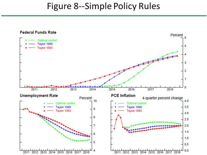
Yellen
also used the FRB/US model to construct the federal funds rate path called for
by the 1993 and 1999 versions of the Taylor Rule conditioned on the same
illustrative baseline outlook used to generate the optimal control path. These paths,
as well as the optimal control, and the various resulting paths for
unemployment and inflation are depicted in Figure 8 of her speech:
The
1993 Taylor Rule calls for the federal funds rate to begin rising in 2013Q2.
The 1999 Taylor Rule calls for the federal funds rate to begin rising in
2015Q1. Optimal control calls for the federal funds rate to begin rising in
2015Q4. More importantly, note that whereas the paths for unemployment and
inflation under the Taylor Rules converge monotonically, under optimal control they
display oscillatory convergence, with both unemployment and inflation
“overshooting” before converging to their long run values.
Now,
it’s true these results were generated with FRB/US and not the Smets-Wouters model.
FRB/US is a somewhat older (1997), large-scale simultaneous equation
macroeconometric model. But because expectations of future economic conditions
are explicit in many of its equations, and adjustment of nonfinancial variables
is delayed by frictions, it too is often described as New Keynesian. The
dynamic adjustment of its aggregate price equation means that, like the Smets-Wouters
model, inflation is dependent on past inflation, expected future inflation and
the current price markup, as well as number of additional variables such as the
unemployment rate, energy prices, etc. And the general effect of monetary
policy shocks on output, inflation and interest rates is quite similar to the
Smets-Wouters model.
Thus
I expect were one to investigate optimal control monetary policy assuming
credible commitment using the Smets-Wouters model, as Bullard mentions the
possibility of in his footnote, one would probably find results similar to
those generated with the FRB/US model assuming it were subject to the same loss
function. To be more explicit, under the same assumptions, an optimal control
path generated by the Smets-Wouters model would very likely exhibit the same
oscillatory convergence pattern of unemployment and inflation as demonstrated with
the FRB/US model.
Thus
it seems to me that the primary issue here is not what type of model should be
used, but what the goals of monetary policy should be. Should monetary policy
be guided by simple rules, such as the Taylor Rules, because in the past, and under
potentially very different conditions, they were considered optimal? Or should
monetary policy be more explicitly guided by the mandates to which it is legally
subject? Or, indeed, should monetary policy be guided by something else
entirely?
Mark Sadowski
Mark Sadowski